Graphic by Danny Taylor

A list of questions to use when reporting on machine learning.

Most importantly, don’t be bamboozled by hype and technical terms, and especially don’t expect that the name of a machine learning method will tell you much about what it does. Everything in machine learning comes down to doing relatively simple things to data (and sometimes involves many relatively simple steps).

While machine learning can sound like computational or mathematical wizardry, scientists should be able to explain and justify their choices, the resulting accuracy rate for prediction, and the pitfalls. Don’t be shy to ask questions about the data on which these models are trained, and the ways in which the scientists assess the models’ validity for future prediction. Here are some suggestions on what to ask:

ON MODELS

1. What prediction model is being used? Is there a way the prediction problem was set up to take account of structure in the problem?

For example, in large scale images, looking at small patches is often a good way to get local information about things like edges. In handwriting recognition, making sure you can rotate the picture a bit and get the same prediction is important. Some of this can make for very cool stories if you can explain it clearly.

2. How sensitive are the models to the choice of methods you used? If the data were slightly different, would the results be similar to what you achieved?

ON METHODS

1. Did you create this method in the hopes of others replicating it using different data sets?

2. As a measurement of success, what is the predictive accuracy that you (the scientist) achieved?
a) How much better is this than what has been done before?
b) What does that measure of accuracy mean in the real world?
c) How reliable is that accuracy over the different test-sets?

3. Will concept drift be a problem in the application? In other words, will the data that emerges over time be consistent with data used to develop the prediction model?
a) Have you (scientist) done anything to try and assess how much of a problem it might be?
b) Have you (scientist) done anything to mitigate its impact or account for how the results might be impacted?

Related Content:

Dr. Stephanie Mathisen of Sense About Science U.K. on “Algorithms and Decision-Making” at the House of Commons

By contrast, the point of machine learning is to predict well. Any attempt to produce a sensible or understandable model is a distinctly secondary consideration. If, for example, the post office takes a picture of a zip code that you scribbled on an envelope and wants to translate that image into letters and digits, it really doesn’t care how the grey-scale value of the 67th pixel affects the likelihood that you wrote a 2—it wants to get the correct character as often as possible. Facebook feels the same way about choosing which advertisements to show you (it wants the one you’re most likely to click on) and an automatic trader only wants to work out which stock will be most profitable. There are a huge range of tasks that are we-just-need-to-predict-well assignments, including many that you wouldn’t naturally think of (Google’s automatic translation is a good example, so is its Go-playing machine) and the methods of machine learning have been successful in completing them.

A side distinction is that while most statistical problems focus on predicting a numeric quantity (e.g. remaining years of a healthy life), the majority of machine learning involves predicting a category: “What letter is this?”, although “How much money will I make on this trade?” is often still relevant. To make these distinctions concrete: imagine the problem of a bank deciding whether to give someone a loan. The bank collects a lot of data on customers (income, age, savings, credit scores, payment history, number of dependents, preferred brand of yogurt—things that are likely to be helpful). A traditional analysis would build several models and report: “Accounting for age and income, the size of the loan that a customer takes out without defaulting increases, on average, by $1,793 for every additional $1,000 of savings.” The $1,793 will often be accompanied by a confidence interval of $1,714 to $1,882.

By contrast, machine learning gives you no such guidance; it simply takes all the data about a new customer and predicts what the loan will be.  More frequently, machine learning will only predict whether the customer will default.

Even this example, however, doesn’t really describe the shift to machine learning adequately. In many cases, categories are the only things that are relevant. For handwriting recognition, you take a picture of a character and ask “What character is this?” There are two things that are very different here. First, there is no number to predict, only whether it’s an a, b, c,… (or possibly 1, 2, 3,…).  Second, the data is a digital image: think of the picture as being made up of a grid of little dots—the “data” that you get out of it is a long list of numbers telling you how dark each dot is.  In this case, there is no understandable relationship between the value of a particular pixel and whether the character is a g.

So how does machine learning do this? The 1,000-foot view is that rather than trying to understand the problem, a computer is fed data about a large number of examples, including everything measurable that might affect an outcome you want to predict, and the corresponding outcomes. The computer then “learns” patterns of “features” (the machine learning term for “measurement” or “covariate” or “predictor variable”) in the data to make a good prediction.

Learning

We’re still using whizz-bang buzzwords here, so how does “learning” actually happen? This is somewhat more prosaic than what occurs in a student’s head in a university lecture theatre. There are a few basic strategies that are used, which I’ll try and describe with minimal mathematics.

Here are four of the most common strategies for machine learning algorithms: nearest neighbors, tree-based methods, neural networks, support vector machines (SVMs). For each, you have data to “learn” and you’ve got an example for which you’re making a prediction (e.g. Will this individual default on the loan applied for?).

Nearest neighbors and example-based approaches. You have data you want to make a prediction for, and in order to do so, you search a larger data set for the example that is most similar (similar has to be defined somehow) to your current data as it relates to the outcome you seek. The outcome of the most similar example is a best guess for the predicted outcome. If I’m a bank trying to decide whether to give someone a loan, I’ll look among my existing customers and find one that’s most similar to the current applicant and see how reliable he or she is. Sometimes the algorithm might look at several “close” examples so that a fluke in the current data doesn’t influence the resulting prediction.

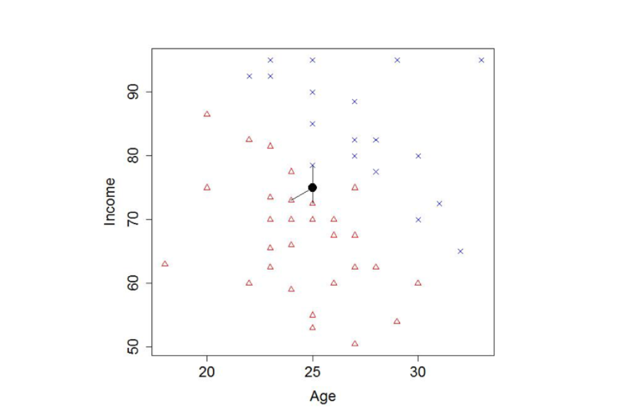
Figure 1. A made-up example of the nearest neighbors method
We try to predict whether someone will default on a loan (red triangles) or not (blue crosses) based on age and income.
For a new applicant (black circle), we have drawn lines to the nearest three examples in our data. Here the majority vote points to a default. In a real-life application, there might be tens or hundreds of features instead of just two.

There are a number of choices to make here: How do you measure “similarity” between examples? How many close examples should you look at before coming to a prediction? Should you give more weight to more similar examples than those that are less similar? Despite these many choices in designing the analysis, the main thrust is to relate the current problem to something from a past experience.

Note that while the idea makes good sense, this method gives you no idea about what might be important in determining whether or not the person is a trustworthy lender. Within machine learning, that’s viewed as rather beside the point.

Tree-based methods “Does the applicant have an income above $30,000? If so, is his or her credit score over 650? Then give that person a loan!” We can encode a series of questions in a tree, which can bring us down to a prediction. If the answer is yes, go left, otherwise go right in the picture below.

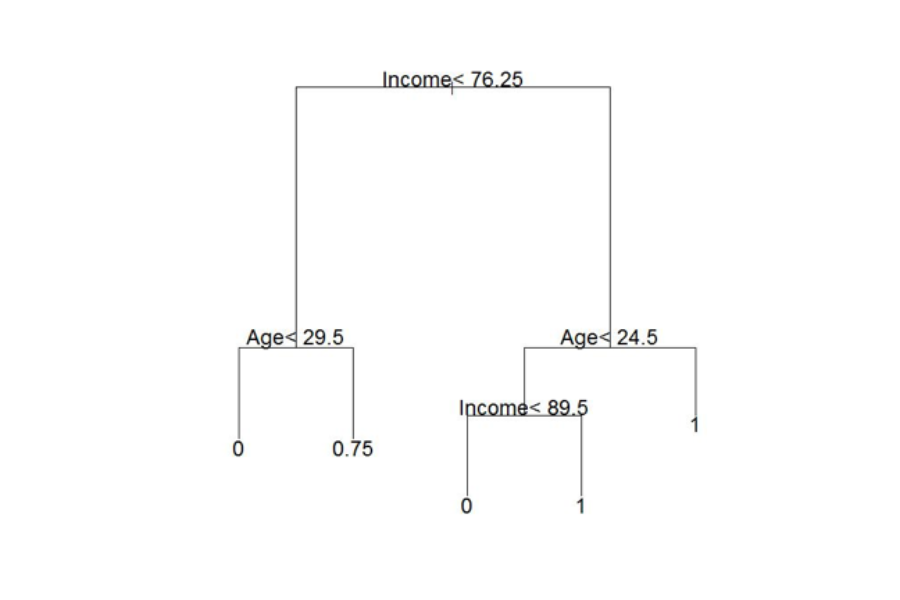
Figure 2. The decision tree for the loan default problem above
At each stage of the flow diagram, we go left if the statement is correct and right if it is incorrect. For this example, age=25 and income = 75. At the top node we go left, then at the second layer we go left again; the result of 0 means that default is likely. 

Methods to obtain trees from data were developed in the late 1970s. To create the top node in the tree, look through all the possible questions you could ask (all the variables you measure and all the values you could use to divide the data along that variable), choose the one that makes the responses as similar as possible for the data on each side of the split. Now, split the data according to the responses to the chosen question: this gives you two data sets (one on each side of the split), each of which tends to have more similar outcomes than the over-all data. Next, try to split up each of the two data sets using the same procedure, and so on.

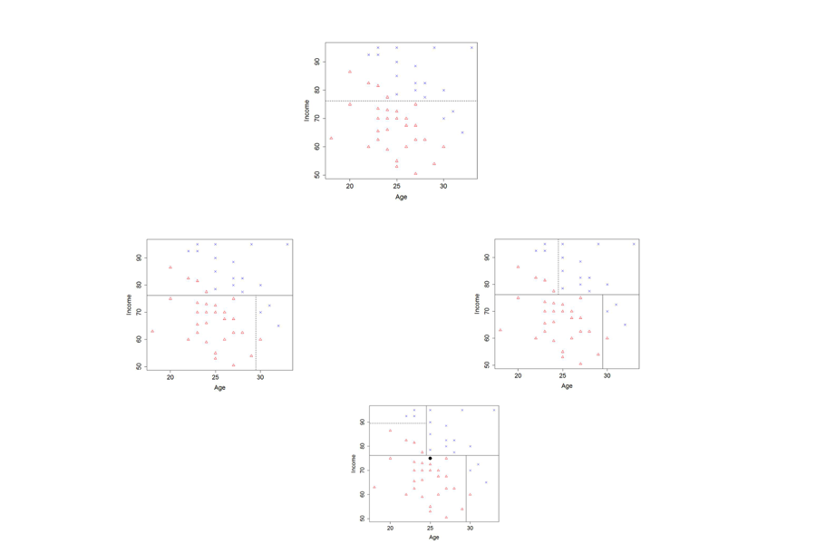
Figure 3. The process of building a tree
We start with all the data (top square), and look for the best vertical or horizontal cut so that each side of the cut is dominated by one response (default or not) or another; in this case at Income = 76.5 thousand dollars per year. We then take the data on one side of the income divide, and split it up again, this time according to age. In the second row, the “bottom” (representing people with income less than 76.5) turns out to be the best split at Age = 29.5 years; the “top” income level is best split at Age = 24.5 years. In the third row, we try to split the “top left” again—this time at Income = 89.5 thousand dollars per year. In each of the resulting regions, we predict the outcome that applies to the majority of the cases in that region. Looking at the new point (represented by a black circle in the third row) we see that the algorithm predicts this person would default. We would get a very different prediction if the first split was at only a slightly smaller value of income, or split at Age = 24.5 years.

Unlike machine learning processes using the nearest neighbors technique, a single decision tree can be understood pretty well, if it doesn’t get too large. You can follow the sequence of decisions by hand.

Unfortunately, trees by themselves perform pretty badly, mostly because they divide up the data so aggressively and can change quite a lot with only slightly different data. A modification of the tree idea, however, has had more success. This involves the creation of “ensembles” of trees, or many trees—usually hundreds—each built using slightly different data. The easiest way to do this is to take a sample from the data set (say about 1/2 of it) and build a tree, then take another sample (some of which might overlap the first) and build a tree, and so forth. Predictions based on the whole data set are derived from predictions made among these samples of data. Each tree makes a prediction and you take the average.

Ensembles of trees routinely perform well. If you go to kaggle.com, which runs prediction competitions, random forests (one type of ensemble, similar to what I described above) provide their baseline performance, which competing teams try to beat. The random forest predictive models are often rated among the best performers.

The single tree picture may be simple to understand, but we can’t easily “understand” how hundreds of trees, all of which are slightly different, result in a prediction. This is characteristic of machine learning methods. The computer figures out the prediction for you, but cannot tell you why it made that prediction, which features in the data it thinks is important, or what might change the prediction it made.

Neural Networks have a completely different mechanism that comes from a loose likeness to biology. In our brains, neurons receive spikes of electrical stimulus from other neurons to which they are connected. When they receive a sufficient stimulus they emit a spike themselves that travels down their axon and stimulates neurons to which they are connected. This is the physical means by which we all think and perceive the world.

Neural networks in machine learning have only the most tenuous connection to these biological ideas, but they are conceived as passing information between simple processing units called nodes (“neurons”).

When a neural network is assigned an image processing task, say, the incoming data is given as a string of values indicating the color of each pixel in the image.  These values are fed to “perceiving” nodes, each of which takes the values and comes up with a score by weighting dissimilar pixels differently. In the biological analogy, neurons attached to cells in the retina of your eye receive a stimulus from each cell, but respond to different parts of the retina or different patterns of light stimulation. The nodes pick out fairly simple patterns: edges, shapes, contrast etc. The scores indicate the strength of match of the pattern that each perceiving node is looking for. This set of perceiving nodes passes their scores on to another set of nodes that combine these together to find larger patterns (“concepts” in machine learning speak), their scores are in turn combined to produce a prediction.

This process applies not just to image processing, but to any task where you start with a set of numeric quantities and want a prediction. The figure below provides the way neural networks are usually visualized (here applied to deciding whether or not to give someone a loan). Inputs start on the left and are fed through a series of nodes. Each node takes the input it is given, computes a score, and passes it along to the next node.

1. In the left-most layer, each neuron is given the features of an example. The neurons each combine these features using their own set of weights and produce a numeric output. Those outputs are then passed on to the second layer.
2. The second layer does not get to see the features directly, instead they get the numerical signals from the first layer. But they do the same thing with these numbers: combine them with their own weights and pass their output on to the next layer.
3. The final (right-most) layer has just one neuron: it takes the signals from the previous layer, combines it with some weights, and uses the result as a prediction.

Notionally, we think of each layer as examining more and more complex “concepts;” however, it is important not to get too carried away with biological analogies, or even this basic interpretation. The neurons in your brain are more complicated than the nodes used in neural networks and can behave quite differently. Even the notion of building up concepts is difficult to see when you look in detail at what a neural network is doing. Another way of thinking about it is that the structure of a neural network is very flexible and can be used to detect very large class patterns if they are found in data.

Traditionally, neural networks, which were developed in the 1980s, had only two layers of nodes: one that combined inputs, and a second that combined the output of the first layer and made a prediction. More recent “deep neural networks” have many layers (from three to thousands depending on the problem) and the structure of the network is often chosen carefully for the problem at hand. In image processing, for example, it is common to enforce the intuition that early layers should learn simple concepts: each input node might only look at a small patch of the image, with the idea that it might detect that there is an edge in that patch; it then passes this on to other nodes which put together several patches to classify the image as a dog, or a computer. The use of “deep learning” (machine learning with deep neural networks) has produced huge improvements in a number of tasks; particularly using images and in speech recognition.

So how does a neural network “learn”? Well, to begin with, the scientist has to set up the structure of the network, say by creating nodes and assigning the connections between them. The goal is to assign weights to connections between the nodes. The computer algorithm looks for the weights that give best performance in a manner not too dissimilar to those used in standard statistical models. There are many more weights than most statistical methods use but basically we search through many values for the weights trying to improve our predictions as we change them. Neural networks have had enormous successes, however, unlike ensembles of trees or nearest neighbors, neural networks require a lot of input from a human. This includes choosing the structure for the nodes and their connections, and fine-tuning the algorithm that looks for good weights. You can get a lot out of neural networks, but you have to spend a lot of time for every new model in order to do so.

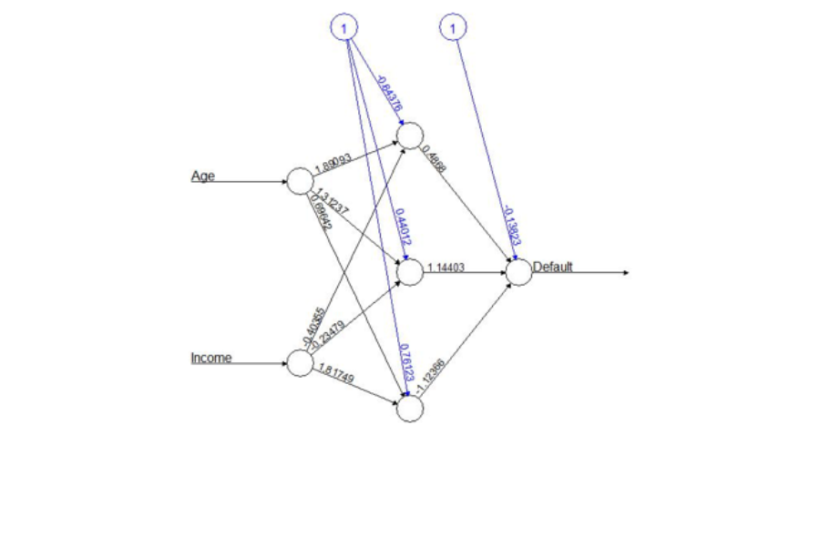
Figure 4. A neural network to predict loan default
The middle layer of nodes (circles) each produces its own weighted combination of age and income and passes that onto the output node which weights the three inputs that it receives to produce a prediction. In modern networks, there are many more nodes in the middle layer, and sometimes several layers.

Support Vector Machines (SVMs). These generally apply to two-way classifications – separating data into one of two groups (good loans versus bad loans for example) – and are the most mathematically motivated. However, there are variations that will predict more than two labels, or a numeric quantity. In a basic sense, SVMs focus explicitly on drawing a boundary between two classes. They try to make sure that points in each class are as far away from that boundary as possible. Think of dividing up territory between two groups and creating the widest ribbon of “no-man’s land” you possibly can in the middle. SVMs do the same thing; the width of the separating ribbon stays the same all the way along the boundary and is referred to as the “margin.” In the picture below, the boundary is a straight line but it is possible to draw boundaries that are more complicated if they need to be.

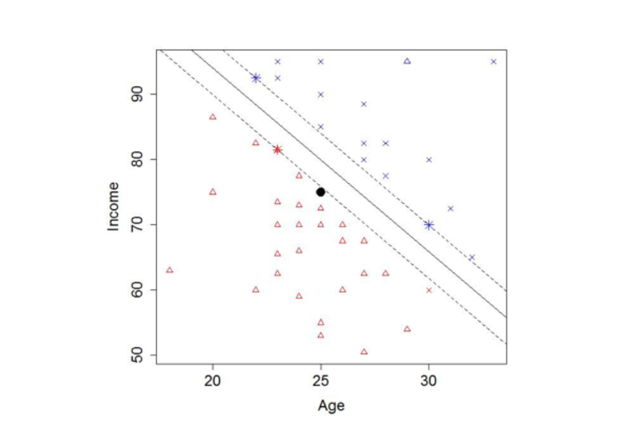
Figure 5. Support vector machine using Age and Income to predict default
The decision boundary is the solid line, while the margin is the distance from the solid to the dashed lines. The starred points are the “support vectors” that determine the decision boundary. For the purposes of making the margin visible, we have removed two points relative to previous examples.

So where does the name Support Vector Machine come from? Well if you try to make your margin as large as possible, the ribbon of no-man’s land will touch only a few of your actual data points—data farther away from the boundary is irrelevant. These are the “support vectors” (the vectors of values that “support” the boundary). The term “machine” may be there to be emotive. For a period of time when SVMs were popular almost anything in machine learning (including ensembles of trees) was labeled a “machine.”[4]

Evaluating a Machine Learning Model

Reporting on machine learning methods is somewhat different from reporting on statistical analysis. There isn’t a quantifiable result (such as, for example, increased heart attack risk) to attribute to a change in a variable (such as increased consumption of processed meat), which we often see in statistical reporting. (e.g. “Eating processed meats three or more times a week increases your chances of having a heart attack by 20%.”) So to some extent, all there is to ask is: “How well does this machine learning algorithm predict”?

Within machine learning, it is standard practice to measure performance by how well the method predicts on “new” data. The reason for this is that machine learning models minimize prediction error on the data they use to “learn.” If some of the response is due to random variability, the method will overfit: it will model patterns in the data that only occur by chance and won’t be present in future data.

To assess future predictive performance, researchers typically split the data into three parts:

1. A training set used to produce the model; at least 50 percent, but sometimes 80 percent of the data, is used for training.
2. A validation set used to choose some aspects of the method, such as how many neighbors to use, how deep the trees or the neural network should be, and what type of separator a support vector machine should have.
3. A test set used to measure predictive performance only after the model has been finalized.

It is now standard practice to report test set performance as the final assessment of how well the model does; however, there are a few things to look out for in this:

Is your test set representative of future data?
The idea of concept drift [5] is that the measurements in your data may shift over time, so you are training (and possibly testing) on data that becomes less representative of the new data on which you will actually employ the model. There is a field called transfer learning that tries to improve future performance in this situation.

Is this an example of “how to do it?”
Or is the model that the scientist has “learned” the final product?lot of machine learning researchers will develop a method for, say, predicting cancer risk, using a particular data set. However, the particular prediction model isn’t being recommended, it’s how to produce the prediction model that the researcher wants to publicize. Someone who wants to build on this research would get their own data, and build their own model. This would then be slightly different from the first model, possibly because the problem is slightly different. This is different from “We have produced this model already and you don’t need to learn a new one.” A good example of a “final product” might be a speech recognition model that Apple uses for Siri. Apple deploys this particular model for everyone and will be interested in how it performs, not how well you might do if you tried to build your own model for speech recognition. By contrast, someone who has developed a decision tree to predict whether an epileptic patient will make high use of emergency rooms in New York might suggest that decision trees do this well; a hospital network in Chicago would then want to build its own decision tree based on the specifics of its data.

Does it reliably produce good predictions?
If someone is recommending a method, rather than a particular model, they should provide some evidence that it can reliably produce good predictions when “learned” with different data. Often this is done by using several different data sets, for several different problems – it’s just prediction after all. If they don’t apply it to different data sets, they should minimally split the data up into three parts several times and observe that predictive performance remains reliable over different splits. Preferably, scientists touting new methods will do both.

Conclusion

There has been a lot of hype about machine learning, partly because all these methods have achieved successes in practical problems. They are used in a wide variety of contexts, from consumer goods, to public policy, to scientific research, to playing strategy games like Chess and Go. Part of the reason they have been so successful is that they can process enormous volumes of data and adapt to complex patterns in data. Machine learning does have its shortcomings though, mainly that it cannot tell a human much about what’s important in the system, nor about uncertainty. However, most machine learning researchers would say the relative importance and/or the uncertainty of the prediction really are beside the point. Freeing ourselves and embracing processes other than traditional statistical methods has allowed for a powerful use of data, and one that isn’t going anywhere anytime soon.

—
[4] Someday I will achieve fame with a “deep neural tree machine”—this will be a variant of nearest neighbors.
[5] This is unhelpfully inconsistent with other naming conventions. “Feature drift” may have been a better term; artificial intelligence started out hoping that machines could learn “concepts” (patterns in data) from which to make predictions.