Examples of elementary
data analysis

Finding an average—on steroids

Basic Explanation. Most journalists understand two important and basic notions of the “average.” There is the median, which involves listing the numbers in order, and picking out the middle number.

For example, the median of the set of numbers—

3, 213, 51, 14, 20

—is 20, because when put in order 20 is the middle number.

The mean, in contrast, involves taking the sum of numbers and dividing by the number of numbers. The mean of 3, 213, 51, 14, 20 is 60.2, because:

An important feature of these two ways to talk about an average is that a median is not very sensitive to outliers, whereas a mean will change a lot if one number is much larger (or smaller) than the other. Moreover, both the mean and the median implicitly regard each number in the list as equally important. At times, this is not the case.

In a variety of contexts, these concepts require quite a lot of thought or context about how to apply them.

Example. Sometimes one has to make a decision about whether to use the mean or the median. Consider the reporting done by the New York Times, in which the paper created a graphic representing the “Educational attainment in each school district” matched against “Parents’ socioeconomic status.”

Each point on the accompanying graph represents a single county, with a single position, horizontally, indicating “Parents socioeconomic status” for that county, and one single position, vertically, indicating “Educational attainment” for that county.

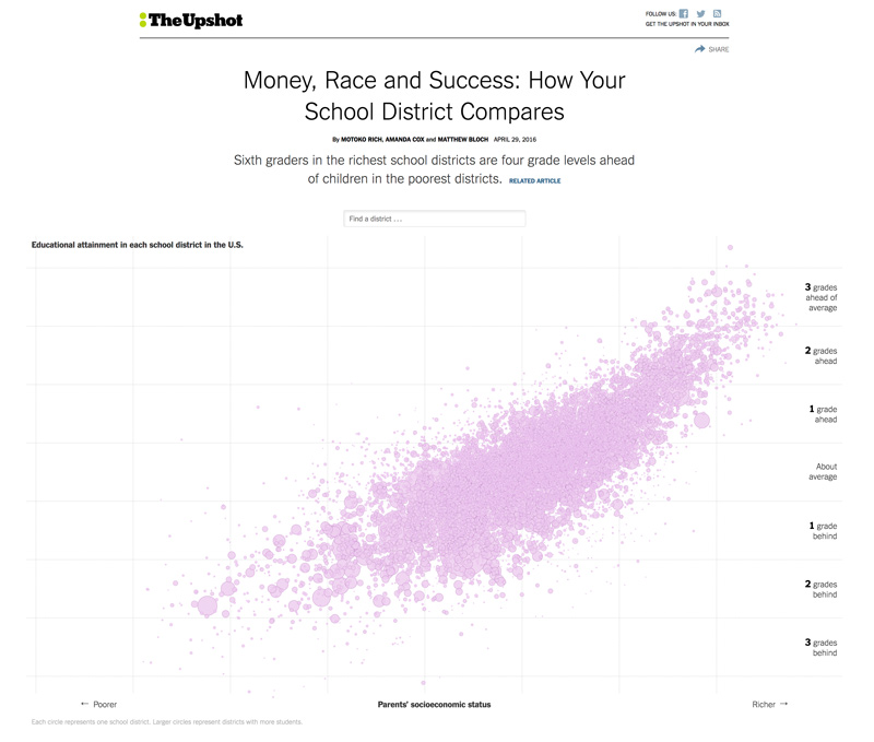
“Money, Race and Success: How Your School District Compares,” New York Times, April 29, 2016 

Clearly some notion of an average should be used to evaluate socioeconomic status, and another to evaluate educational attainment; but how?

The Times used “median income” as part of its measure of socioeconomic status, rather than the “mean income.” The median is the level of income at which half of people make more, and half make less. This decision makes sense, since the median is not sensitive to outliers, specifically, people with relatively extreme wealth. If a few wealthy people move into a relatively poor school district, their income will change the mean income, but it won’t grossly impact the median income.

The “educational attainment” score is measured in part part through the National Assessment of Educational Progress (NAEP) test results. The NAEP offers scaled scores in each subject, and these are mean scores on a scale of 0-500 in each subject, rather than median scores.

In this case, either a mean or median test score would be appropriate, as the data will generally fall into a “bell curve” in which the mean and the median agree. Note that the test scores are capped at how high or low they can go, which implies that the mean (average in the traditional sense) will not be impacted grotesquely by outliers. One reason that standardized tests often favor a mean as opposed to a median is that a typical measure of variance, the standard deviation, calculates how far away data are from the mean (rather than the median).

Example. In some cases, how to compute an average isn’t obvious. If you have data on the high school graduation rates among 315 public high schools in the state of Virginia, how would you find the actual rate of graduation?

The problem is that one school might have a four-year graduation rate of 98 percent among 3,000 students, while another has a graduation rate of 86 percent and has 800 students (we don’t worry here about whether the number of incoming students changes each year, but rather take the numbers at face value). If you average the numbers 98 and 86, you would obtain a score of 92 percent ((98+86)/2 = 92). But this calculation seems to be misleading; the school with 3,000 students has more students and should somehow count more.

This situation illustrates the need for a weighted average of these two values. All together, there are 3,800 students. Of these 98 percent of 3,000 graduate on time, or 2,940 students. At the second school, 86 percent of 800 students graduate in 4 years, or 688 students. Together there are 3,628 students who graduate on time, out of 3,800 total. That’s a much more impressive graduation rate of 95.5 percent.

To carry this out more systematically, rather than adding up 98 and 86 percentages and then dividing by 2, we “weight” the 98 and the 86 to match up with the percentages of the population they pertain to. In this case, 3,000 students out of 3,800 are in the school with a 98 percent graduation rate; as a proportion 3000/3800= .789 (or 78.9 percent). Similarly, the school with the lower graduation rate has a different proportion of the students, 800 out of 3800 students, or 800/3800=.211 (21.1 percent). Those proportions are the “weights” we use to find the weighted average:

.789×.98 + .211×.86= .955

When using the data of 315 schools, rather than two schools, you will want to use an Excel chart to keep track of each term in a sum of 315 items. Here are the steps:

1. Each row should correspond to an individual school. Enter in Column A the names of all the schools.

2. In Column B: enter the percentage of students graduating in each school

3. Column C: enter the size of the student body in each school.

4. At the bottom of Column C, find the total number of students by summing all the previous entries of Column C. This total number will be important to find the proportion.

5. Column D: divide the size of the student body (from the corresponding cell in Column C) by the total number of students. This is the proportion of all students who attend each school.

6. Column E: multiply the proportion by the percentage of students graduating.

7. Add up the entries of Column E. This is the average graduation rate!